
by Jonathan Kujawa
Nearly four years ago here at 3QD we talked about how Euler became interested in a trifling little puzzle in 1736. He asked if it was possible to take a walk through the city of Königsberg, Prussia and cross each of its seven bridges once and only once. It seems like a silly thing to spend your time on and is obviously of no use to anyone. My former senator would have an aneurysm at the idea of funding such research. Fortunately for us, Frederick the Great was more of a visionary.
Being no slouch, not only did Euler solve the problem (spoiler: it’s not possible), he invented two major fields of modern mathematics in the process. Four years ago we followed one of those rabbit holes and were led to the field now called topology. It is the study of geometry when you don’t care about angles, distance, and the like. Topology is a rich and exciting area of modern research with all sorts of applications. It leads to subway maps, the use of homology to study the structure of huge data sets, motion planning for robots, and gives us that one easy trick for solving labyrinths like a Theseus.
The second rabbit hole is the one we follow today. It leads to another area of modern mathematics now called graph theory.
In mathematics, a graph is nothing more than a collection of nodes and connections between them (sometimes called vertices and edges, respectively). Graphs can be drawn where each node is a dot and each connection is a line connecting the corresponding dots.
For example, the Petersen graph:
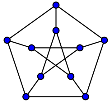
It has ten vertices and fifteen edges.
In Euler’s mind the various islands and districts of Königsberg were the nodes and the city’s bridges were the edges. In the modern era we see graphs everywhere we look: computers and networks, customers and their purchases, countries and their alliances, Facebook or Twitter and those you follow, Kevin Bacon and the other actors in his films, scientific researchers and their collaborators,… Whenever you have things and connections between them, you have a graph. What started out as the silliest of questions is now at the center of many modern applications of mathematics.
There are a couple of important things to keep in mind when thinking about a graph. The first is all we care about are the nodes and the edges which connect them. Drawing a picture of a graph is for convenience only. There are many, many ways of drawing any given graph. They may look radically different but, as long as all connections between nodes are the same, its the same graph. For example, here’s another picture of the Petersen graph:
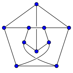
Also, since we only care about the connections between nodes, when we draw edges crossing each other we always think of one edge going over or under the other. While they may cross, they don’t actually touch each other. The second picture of the Petersen graph shows this convention. Since we don’t care which edge goes over and which goes under we often draw the strands crossing (like in the first picture of the Petersen graph).
After drawing a number of graphs you soon realize some can be drawn without any crossings if you are clever enough. It’s not so obvious, but if you move around the nodes just right you can draw the same graph but with none of the edges crossing:
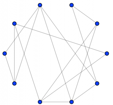
It’s a fun puzzle to figure out how to redraw this graph so it no longer has crossings. In fact, there is a great free online game called Planarity where the entire goal is to solve puzzles of this kind.
A graph which can be drawn without crossings is called planar. While the graph above is planar, try as you might you’ll have little luck drawing the Petersen graph without crossings. Indeed, after a few evenings of drinking scotch and drawing the Petersen graph in various twisted ways, you might just start to believe it can’t be done.
This raises the question of which graphs are planar, which are not, and how can you definitively tell which is which? An amazing early result of graph theory is the famous Wagner’s theorem. It tells you exactly which graphs are not planar.
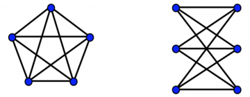
For example, in the first picture of the Petersen graph if we contract the edges connecting the inner star to the outer pentagon we uncover a K5. Thanks to Wagner we know every drawing of the Petersen graph must have crossings.

Wagner’s theorem is the kernel to several “impossible puzzles”. The most famous is the Three Utilities Puzzle: can you connect three houses to the gas, water, and electric companies without the connections crossing? This is a great one to give to nieces and nephews. Just don’t forget to tell them about Wagner’s theorem and K3,3 when they give up in frustration!
Long-time readers will remember when we ran across non-planar geometry. It isn’t always old fashioned geometry in the plane we care about. Indeed, the Earth is a sphere and when we lay pipeline, internet cables, and plan airline flights, we know to take this into account. When your family tires of drawing in the plane, have them try the Three Utilities Puzzle on a globe. It turns out that you still can’t solve the puzzle on a sphere but you can solve it on a donut. But a donut and a coffee mug are the same to a topologist. This means you should be able to solve the Three Utilities Puzzle on a coffee mug. And indeed you can. The fine folks at Maths Gear sell a mug so you can try it at home. Tamás Görbe recently posted a video showing you can also solve the Four Utilities Puzzle on a coffee mug.
Of course in the real world there is more to networks than who is connected to whom. You might want to label your edges with distance if it is a rail network. Or rate your Facebook friends on a scale of 1 to 5 rating (frenemy to besty?). Or the cost of building each segment of pipeline. Mathematicians say a graph whose edges are labeled is colored. If you only need a couple of labels, it’s visually appealing to use actual colors like red, blue, and green. For more complicated or practical labeling schemes you might have to switch to boring ol’ numbers.
This may ring a bell for truly dedicated 3QD readers. A long, long time ago we ran across Ramsey’s marvelous theorem. In it, Ramsey proved structure and order inevitably emerge as networks grow in size. A little more precisely, he showed if you have a finite list of allowable colors and any fixed graph in mind, then however you choose to color a sufficiently large graph you can’t help but create a monochromatic part of the graph which matches the graph you have in mind.
Alternatively, instead of coloring edges you could color the nodes. Maybe each node is a person and you label them by the country they are from. Or maybe they are airports and you label them by how many flights they can handle.
Let’s say for some reason you want it so anytime two nodes are connected by an edge you would like them to have different labels. For example, in a triangle you would need three different colors since every pair of nodes is connected. However, in a square you still only need three colors if you’d like to label the connected corners with different colors.
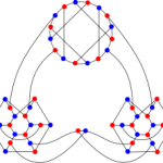
Let’s call a coloring of the vertices of a graph where any two connected vertices always have different colors a Good Coloring. If I have more colors than vertices, then I can always find a Good Coloring. Just color every node a different color and then it doesn’t matter who is connected to whom.
The real challenge is to find a Good Coloring which uses the fewest possible colors. This fewest number is called the chromatic number of the graph. One way to think about the chromatic number is as a measure of the connectedness of the graph. Generally speaking, the more edges a graph has the higher the chromatic number.
For example, the triangle and square both have chromatic number 3. What about other graphs? Well, K5 has chromatic number 5 (every vertex is connected to every other vertex so we can’t use a color twice). On the other hand, the Petersen graph has chromatic number 3. Since it contains triangles, 3 is the lowest it could be. The trick is to find a Good Coloring which uses 3 colors and no more.
As you might imagine, computing the chromatic number of a graph is computationally difficult for large graphs. A brute force search grows exponentially as you increase the number of vertices. One favorite trick of mathematicians is to solve a problem by figuring out how to break the problem into smaller pieces. Or, said differently, if you know how to solve it for smaller pieces and how to put the pieces together, you can get the solution in larger cases.
This brings us to Hedetniemi’s Conjecture on chromatic numbers. In 1966 Hedetniemi made a now-famous conjecture which was finally resolved just this May. His conjecture involves graphs which are made out of two smaller graphs in a way which I’ll explain by an example. Say you have a group of heterosexual couples. You can make a graph we’ll call M where the nodes are the men and there is an edge connecting each pair of men who are friends. Similarly, we can make a graph we’ll call where the nodes are the women and each edge connects a pair of women who are friends. Starting with these two graphs we can build one graph for the couples which we’ll call C. Each node of C is one couple, and there is an edge between two couples if and only if there was an edge between the men and an edge between the women. That is, two couples are friends if and only if the men are friends and also the women are friends.
Taking any two graphs M and W you can use the same rule we used above to make a new graph C. It is not terribly difficult to see the chromatic number of C is always smaller than the chromatic numbers of M and W [3]. Based on examples Hedetniemi conjectured the chromatic number of C is actually always the smaller of the chromatic numbers of M and W.
Over the years people verified Hedetniemi’s conjecture in lots of special cases. Certainly the evidence was in its favor. Then lightning struck. On May 6th Yaroslav Shitov put a three-page paper on the ArXiv in which he showed how to construct counterexamples to Hedetniemi’s conjecture! He gave a machine which constructs graphs M and W such that the corresponding C has chromatic number strictly smaller than those of M and W. Shitov’s paper is slated to appear in the top journal of mathematics, the Annals of Math.
There is another amazing result about chromatic numbers I have to mention. Given n colors and a graph, you can ask how many Good Colorings you can make using those n colors. For example, for the triangle and n=2, there are 0 Good Colorings, but when n=3 there are 6 Good Colorings. If n is greater than 3, then there are exactly n(n-1)(n-2) Good Colorings [4]. You might notice this formula works for n=1, 2, and 3 as well. You might even notice this formula is a polynomial in the variable n. It is amazing and true that for any graph the number of Good Colorings when you have n colors is always a polynomial in the variable n. This is called the chromatic polynomial of the graph.
All of this only scratches the surface of graph theory. Lots of exciting work is going on a mere 380+ years after Euler started it all!
[1] Image borrowed from here.
[2] “K” because they are the komplete graph (i.e. has all possible edges) on 5 vertices and on 3 and 3 vertices, respectively.
[3] If you have a Good Coloring for the men’s graph, you can use the same coloring for the couples graph. Since there is an edge between two couples only if there is an edge between the men, a Good Coloring for the men will still be a Good Coloring for the couples. Ditto for the women’s graph.
[4] You can pick any of the n colors for the first node, any of the remaining n-1 colors for the second node, and any of the remaining n-2 colors for the third node.