
by Hari Balasubramanian
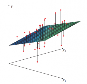
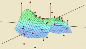
Optimization – the search for the best among many – is at the heart of the statistical and machine learning models that get used so extensively these days. Take the simple concept that underlies many of these models: fitting a mathematical curve to data points, better known as regression. In the simplest two-dimensional case, the curve is a line; in three dimensions, it is a plane, as seen in the figure. Among all possible planes – there are infinitely many of them, obtained by changing the angle and orientation: imagine rotating the plane every which way – we would like the one that passes ‘closest’ to as many of the data points (shown in red) as possible. Thus regression, often called the workhorse of machine learning, is really an optimization problem.
It turns out that optimization is fundamentally connected to even basic statistical quantities. Common statistics we we now reflexively use to summarize data – means, medians and percentiles – are themselves answers to certain optimization questions. We are not used to looking at them in this way.
Let’s take the average or sample mean, which, despite its obvious limitations, everyone turns to first. Suppose we have five numbers in a sample: 3,4,5,8 and 12. The sample mean is given by the straightforward calculation:
(3+4+5+8+12)/5 = 6.4
But there is another way to think of the sample mean: as the optimal answer to the following problem. We seek to find the x that minimizes (produces the lowest value of) the sum of the squared difference between x and each observation in the sample. Mathematically, we can write the function as:
(x-3)2 + (x-4)2 + (x-5)2 + (x-8)2 + (x-12)2
At what value of x does the function have its lowest value? In the figure below, the horizontal axis shows the values that x can take (I restricted myself to the range of the data points, 3 to 12). The vertical axis shows value of the sum of squares function corresponding to each value of x.
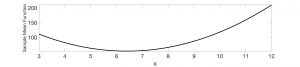
We see that the function follows a U-shape with the lowest/best value, x=6.4, occurring at the bottom of the U. Simple high school calculus – finding that point on the continuous curve at which the derivative is 0 – will yield the same answer. In fact, the formula for the mean, adding up all the sample values and dividing by the total number in the sample, can be derived using such calculus.
§
If this was Stats 101 and too easy, then here’s a more intriguing question:
What kind of function does the sample median optimize?
The median of course is the middle number in a sorted sample: 5 in our example. (If the sample size is even, it is the average of the middle two data points.)
It was only last year that I learned – to my great surprise: somehow this hasn’t fully sunk in and continues to fascinate – that the median is the x value minimizes the sum of the absolute difference between x and each data point in the sample:
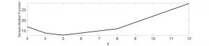
|x-3| + |x-4| + |x-5| + |x-8| + |x-12|
The operator || converts negative differences into positive ones (otherwise we would have some positive differences and some negative ones and we can’t be sure what their sum means).
As an example, when x =3:
|3-3| + |3-4| + |3-5| + |3-8| + |3-12| = 0 + 1 + 2 + 5 + 9 = 17
When x =5:
|5-3| + |5-4| + |5-5| + |5-8| + |5-12| = 2 + 1 + 0 + 3 + 7 = 13
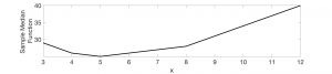
If we plot values of the function for the median (vertical axis) against the values of x (horizontal axis) we get the following figure. Notice that the minimum occurs exactly at x=5 as we’d expect. Also notice that the function, unlike the sample mean case, is not smooth anymore – rather, it is broken into linear segments, with the slope of each segment changing as soon as a data point is encountered. Unlike the sum of squares, which produces a smooth curve, we can’t use calculus so easily when a function is fragmented like this.
The distinction between the function that the sample mean minimizes and the function the median minimizes is only this: in the former case we squared the values while in the latter case we calculated the absolute value. But this distinction turns out to be vital: squaring makes the optimal answer sensitive to distant points, also called outliers, while the absolute difference makes the optimal answer insensitive or robust to distant points. It’s a sudden and unexpected shift.
To see this visually, suppose that the sample changed from 3,4,5,8,12 to 3,4,5,8, 24: that is, the largest value in the original sample, 12, doubled to become 24. The two figures below which plot the sample mean and median functions.
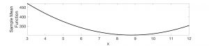
The more distant a point is the greater the influence it exerts on the sample mean: we see that the sample mean has moved to the right. The new minimum occurs at x=8.8. No surprise there.
But the absolute deviation function also adds up the difference between x and each data point. Because one of the data points is now 24, one would expect the optimal x value to shift to the right – but somehow it doesn’t! The values of the function have changed, however the minimum still occurs at x=5. When the sample size is odd, the point that splits the sorted data equally on either side of itself – the very definition of the median – always turns out to be optimal.
Everyone knows that the median is insensitive to outliers. But were you aware of the outlier-insensitivity property of the absolute deviation sum and its link to the median? I certainly was not even though it’s been around for a while. Sometimes stumbling onto simple stuff that one has missed can create a lot of joy!
What applies to the median also applies to other percentiles – after all, the median is nothing but the 50th percentile. We can take the function for the median and tweak it to obtain functions whose minimum value occurs at a certain percentile. Instead of finding the middle point, by weighting the absolute differences adequately, the function can be adjusted to give, say, the 2nd largest point (20th percentile) or the 4th largest point (the 80th percentile).
Implications for Curve-Fitting
We see now that the mean, median and percentiles have their own unique ‘error’ function which they minimize.
Error functions are key in modern machine learning where the goal is to create an optimal curve that fits data points. The distance of each data point from the curve tells us something about the magnitude of the error and thereby the quality of the fit. By far the most commonly used measure of fit is the squared sum of the distance of each data point from the curve. We would like the optimal curve that minimizes this squared error function.
Squared error is so common in modern statistics and machine learning that it is taken for granted. Why is it so popular? I came up with the following reasons. First, squaring shows up in Euclidean distance calculations and in physical laws – Newton’s law of gravitation and Coulomb’s law – so there is a legitimacy that comes from the natural world. Second, the square function penalizes distant points more heavily and that makes sense (but why raise them to the power of 2 and not to the power of 4? Perhaps power of 4 is overdoing the penalty.) Third, in the case of multiple linear regression – still one of the widely used models – squared error functions produce smooth U-shaped profiles, making the application of calculus, and therefore computation, easy. This last point is the important because it allows regression estimates for very large datasets to be obtained at the click of a button. This is why squared error is the default choice in most software.
But when we minimize sum of the squared error, what we will get is a curve that gives us the best possible prediction of the mean of the variable of interest. The problems that the sample mean has carry over to this mean-curve. Outliers can now have a big influence on the shape of the curve.
If you don’t want outliers to have such a big influence you could find the curve that minimizes the sum of the absolute distance of each point from the curve. Such a curve will be the best possible median curve. And because it is a median curve, it will be insensitive to outliers. If the data changes, the median curve is more likely to remain steady or robust compared to the mean curve. Similarly, by weighting the absolute deviations adequately, you could fit, say, a 10th percentile curve or the 90th percentile curve. Sometimes percentile curves can be revealing: factors that predict the 20th percentile of a variable may not be the same as the ones that predict the 50th or the 80th. And a mean curve may miss these nuances entirely. One downside of median and percentile regression curves, however, is that they are not as easy to compute. This is primarily because median and percentile error functions are not smooth: they are fragmented into linear segments and therefore we can’t use calculus like we did for mean curves. That said, it’s not hard to find specialized algorithms that will give you percentile regression curves.
All this is getting a little abstract — I am leaving out specifics in the interest of keeping the column accessible.
My point is that subtle changes in the error function can alter how quickly we can compute the results, what the results mean and how we interpret them. That’s obvious, you might say, but it’s worth reiterating given the hype that surrounds predictive modeling these days. All it takes is to select a few dozen columns in a spreadsheet with a sleight of hand, click a few buttons and we get inundated with a sequence of summary estimates and graphs of a regression model. Sometimes the entire process is automated, part of some invisible algorithmic loop. But unless a user has thought deeply about the underlying theory – and even as an academic trained in probability models, I frequently find myself challenged – he or she isn’t always aware, indeed does not have the time to be aware, of how the final results were generated and the small details that make a big difference. The choice of the error function, of what exactly is being optimized, is one of those details.